Beta's memory length in weighted least squares regression
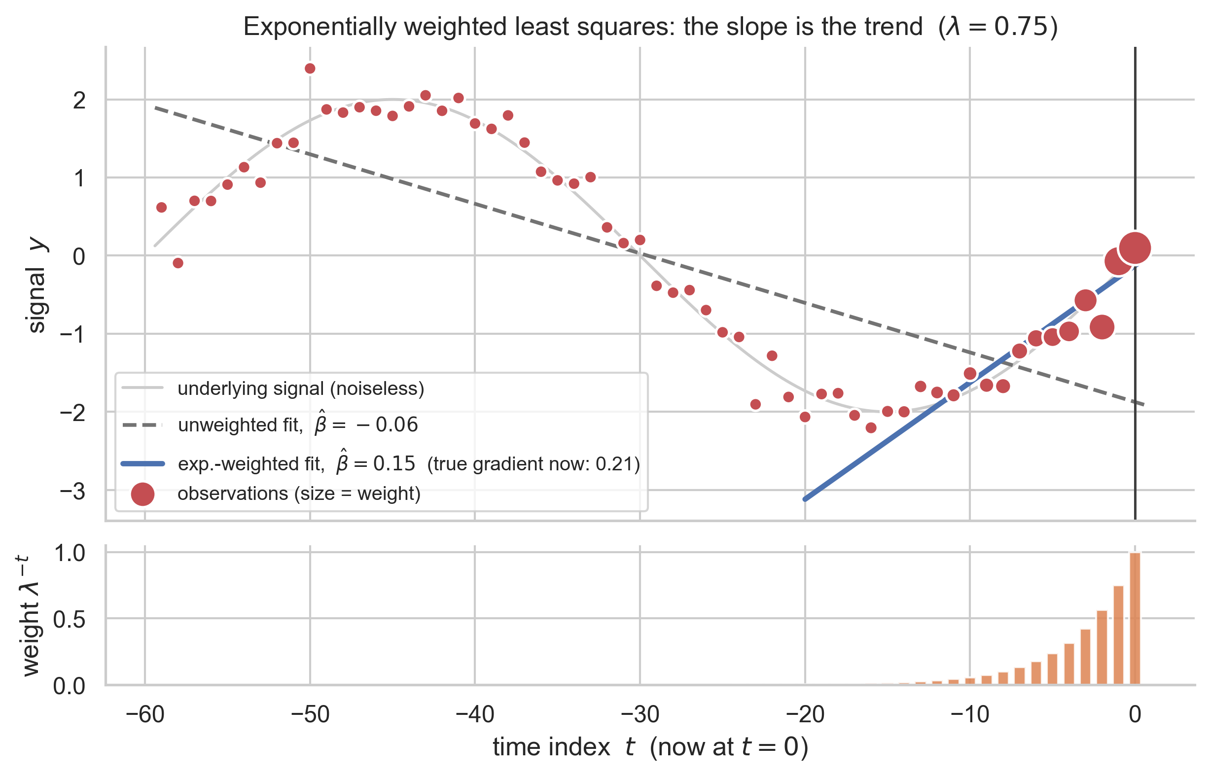
You can use least squares regression to estimate the trend of a signal. If your inputs are time indices, your target is the signal itself, then the regression coefficient \(\beta\) is the gradient of the best fit line.
This means that if you do weighted least squares, weighting recent data more highly than old data, you are in effect calculating the gradient of the signal. The simplest alternative is rise-over-run: the value now minus the value from some chosen time ago, divided by the gap. Noise in real time series prevents that from working well.1 Weighted regression instead uses all the data, giving a smooth estimator of the gradient that is less impacted by very short term deviations, with the choice of weights as the dial controlling how we estimate the trend.2
If I do a vanilla rise-over-run calculation I know exactly what my window size/lookback period/memory length is: if I look at the signal now and compare it to the value of the signal 1 minute ago, I know I am looking at the signal over a 1 minute history. Ok, but if I am trying to estimate trends using this regression approach, what is my memory then?
What I want to tell you about is that the standard memory lengths for weighted linear regression are for the estimate of the level, the value of the signal itself, and that if we are calculating a trend we need to do a slightly different calculation. The punchline is:
For exponential weighting the trend memory length is about 1.8 times longer than the vanilla memory length. (Exactly, it is \(6^{1/3} \approx 1.817\) times longer.)
For example, if you get a new datapoint every hour, \(\lambda = 0.9\) gives a level memory of 19 hours — but a trend memory of about 35 hours.
Some Notation
Let’s add a bit of notation here. We are given \(n\) pairs of values \(\{(x_1, y_1), (x_2, y_2), \ldots, (x_n, y_n)\}\) and we model the relationship in our data as
\[y_i = \alpha + \beta x_i + \epsilon_i,\]where \(\epsilon_i\) is independent and identically distributed noise with variance \(\sigma^2\). In weighted linear regression we weight each datapoint by a factor \(0 < g_i \leq 1\), and we aim to find the \(\alpha\) and \(\beta\) that minimise the weighted sum of squares,
\[\alpha^*, \beta^* = \underset{\alpha,\beta}{\arg\min}\left(\sum_{i=1}^n g_i\left(y_i - \alpha - \beta x_i\right)^2\right).\]One reason for weighting is that some datapoints are viewed as being more important than others to regress accurately at — these are given higher weights.
Applying this to a time series, \(x\) will be the times at which we gain observations and \(y\) the signal. We want local, denoised estimates of the current gradient — we are assuming that the linear model holds only locally — and it is natural to enforce this locality by giving to recent observations high weight and giving to older observations a low weight.
Things are made somewhat simpler if all our observations come at regular intervals. We can then directly identify \(x_i = i\), so \(i\) is simply the time index of the observation. We restrict ourselves to this case.
Exponential weights
Exponential weighting is the obvious go-to: we give the most recent observation weight \(1\) and each observation further back in time gains a factor of \(\lambda\),
\[g_i = \lambda^{t-i}, \qquad 0 < \lambda < 1,\]so the further back in time you are the greater the power \(\lambda\) is raised to. Under this rule, we pay more heed to recently gathered data. (Note that when a new observation comes in it’s not just that we add it to the analysis and do an update; we also retrospectively down-weight all previous data by a factor of \(\lambda\).)
(For the level, this is exactly equivalent to an exponentially weighted moving average: fitting just a constant with these weights gives the weighted mean, which obeys the familiar EWMA recurrence \(\bar y_t = \bar y_{t-1} + (1-\lambda)\left(y_t - \bar y_{t-1}\right)\).)
It’s a standard result that the memory length of an exponentially weighted moving average is
\[t_{\mathrm{mem}} = \frac{1+\lambda}{1-\lambda}.\]Where does that come from? You can get it in a bunch of different ways, but within the regression framework the recipe is to calculate the variance of the weighted estimator as a function of \(\lambda\) and compare it to the variance of a sliding window estimator. The window length for the sliding window variance that matches the weighted value’s variance is the memory length of the weighted value.
Doing this (the variance results are derived in the appendix; both are simple geometric sums): the exponentially weighted mean has
\[\mathrm{Var}(\bar y_\lambda) = \sigma^2\,\frac{\sum_i g_i^2}{\left(\sum_i g_i\right)^2} = \sigma^2\,\frac{1-\lambda}{1+\lambda},\]while a sliding-window mean of \(N\) points has variance \(\sigma^2/N\). Matching the two,
\[\frac{\sigma^2}{N} = \sigma^2\,\frac{1-\lambda}{1+\lambda},\]and so we get that the matching \(N\) value is \(t_{\mathrm{mem}} = (1+\lambda)/(1-\lambda)\), as expected. This approach comes from Brown (1963), Chapter 8 (pp. 106–111), which is also where the familiar smoothing-constant dictionary \(1 - \lambda = 2/(N+1)\) lives.
You can also get this value without computing any variances at all, by matching the average age of the data under the two weighting schemes (that derivation is in the appendix).
Memory length of the trend
What is the memory length of this gradient estimator? More technically: what is the look-back window for an unweighted estimator such that that estimator has the same statistical properties as the decaying estimator? The question becomes concretely: for a given \(\lambda\), for what window length \(N\) do the variances of the two \(\beta\) estimates match?
So we follow the same broad recipe as for the level, but now we are estimating the variance of the regression coefficient beta.
You get (derivation in the appendix; we work in the limit of a long history, \(t \to \infty\), where all the running sums in the estimator saturate at certain values and the estimator reaches its steady state):
\[\mathrm{Var}(\hat\beta_\lambda) = \frac{2(1-\lambda)^3}{(1+\lambda)^3}\,\sigma^2,\]while for the sliding window the textbook OLS result is \(\mathrm{Var}(\hat\beta_{\mathrm{OLS}}) = \sigma^2/\sum_i(x_i-\bar x)^2\), and for \(N\) equally spaced points \(\sum_i (x_i-\bar x)^2 = N(N^2-1)/12\) (also in the appendix), so
\[\mathrm{Var}(\hat\beta_{\mathrm{OLS}}) = \frac{12\,\sigma^2}{N^3 - N}.\]So working it through, by matching the variance between a sliding window and the weighted approach, we get
\[t_{\mathrm{mem}}^3 - t_{\mathrm{mem}} = 6\left(\frac{1+\lambda}{1-\lambda}\right)^3.\]For large values of \(t_{\mathrm{mem}}\) we can drop the \(-t_{\mathrm{mem}}\) term (in the appendix we show this is very accurate for \(t_{\mathrm{mem}} \gtrsim 5\), i.e. essentially any \(\lambda\) you’d use in practice),
which we can rearrange to get the memory length:
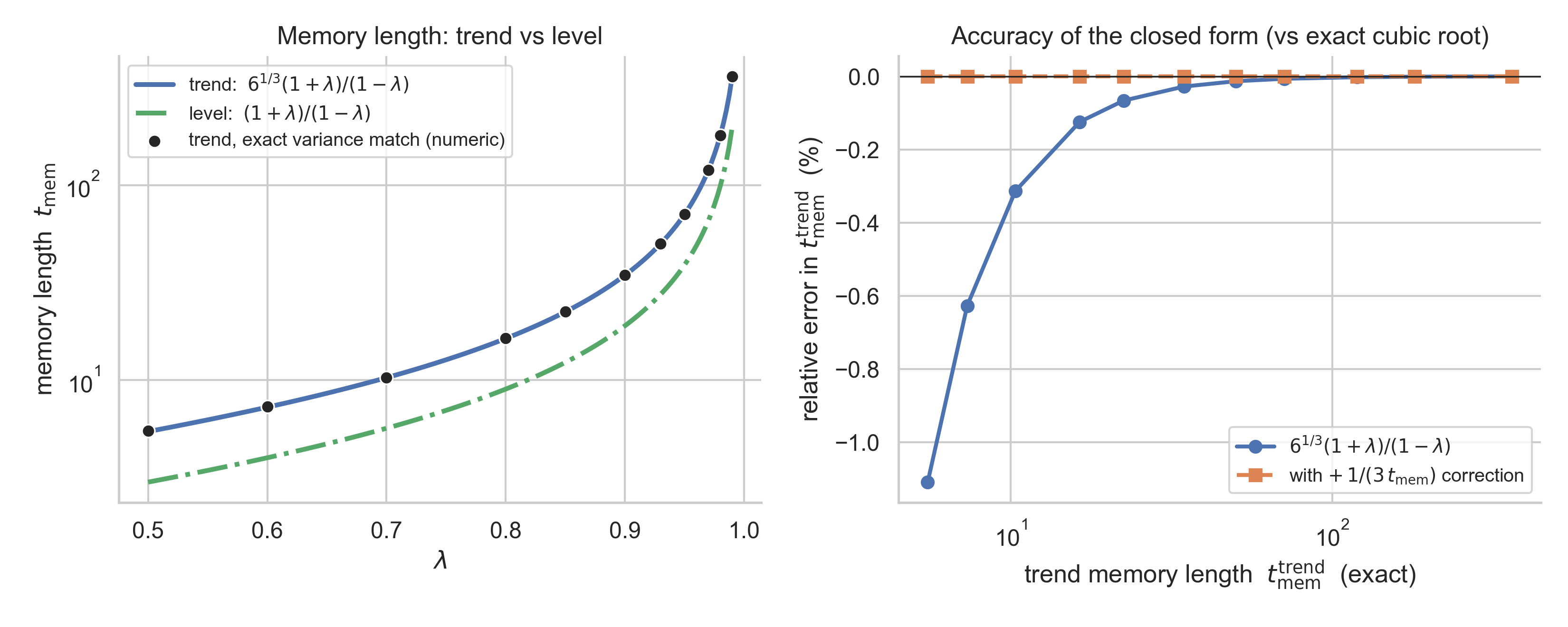
\[t_{\mathrm{mem}}^{\mathrm{trend}} = 6^{1/3}\,\frac{1+\lambda}{1-\lambda} \approx 1.817\,\frac{1+\lambda}{1-\lambda}.\]The cube root comes from the variance of our timesteps, and results in a simple scaling of the ‘level’ result: a mean has variance \(\propto 1/N\) but a slope has variance \(\propto 1/N^3\), because \(\sum(x_i-\bar x)^2\) grows like \(N^3\). The \(6^{1/3}\) is just \((12/2)^{1/3}\) — the 12 from the OLS slope variance, the 2 from the weighted one.
Here is the variance-matching picture, with simulations confirming the algebra:
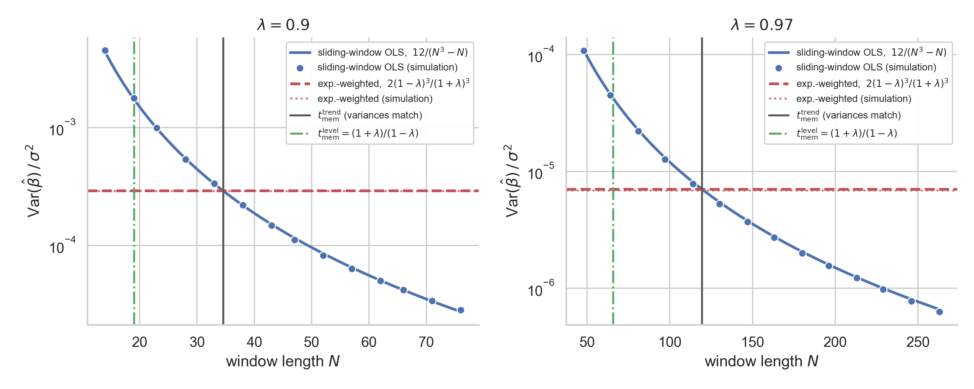
The sliding-window slope variance (blue) falls as \(\approx 12/N^3\); the exponentially weighted slope variance (red) is a horizontal line for fixed \(\lambda\); the window length where they cross is the trend memory — \(1.817\times\) the level memory (green).
Conclusion
When I first dug out these results I didn’t have a clear grasp of why the variance of the gradient is different from the variance of the value. I think there are two helpful views.
First, think about what goes into a vanilla rise-over-run calculation; it’s the value now minus the value from some time ago. Under the hood something like that has to be happening in the statistical estimation, we are adding some values and negating some others.
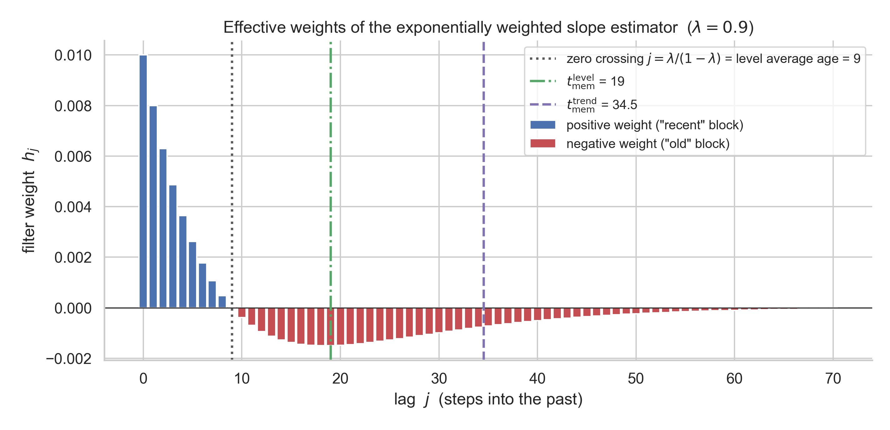
If you write out \(\beta\) as a linear filter, you get \(\hat\beta_\lambda = \sum_{j\ge 0} h_j\, y_{t-j}\), so the effective weights are
\[h_j \;\propto\; \lambda^j \left(1 - (1-\lambda)(j+1)\right).\]This crosses zero at the average age of the data (the centre of the equivalent vanilla window). The negative ‘lobe’ is deepest at the vanilla memory length itself with weights going well beyond that. This naturally increases the memory length over the level estimator: we care (negatively) about these longer-ago data points.
That these weights sum to zero is also why the estimator ignores the level entirely, as a gradient should.
Secondly, \(\Beta\) is a covariance by construction. The slope estimator is the sample covariance of the signal with time, divided by the variance of time: \(\hat\beta_\lambda = \frac{\mathrm{Cov}_g(x, y)}{\mathrm{Var}_g(x)}\), while the level is just a (weighted) mean. That gives the two memory calculations different denominators. The variance of the mean is \(\frac{\sigma^2}{N}\), but the variance of the slope is \(\frac{\sigma^2}{N \, \mathrm{Var}(x)}\). The variance of the (uniform) ticks matters, and a window’s tick-variance grows like \(N^2\). With \(N\) points we get another factor of \(N\), so \(N^3\) overall. The cube root in the memory length comes simply from this.
References
- Brown, R. G. (1963). Smoothing, Forecasting and Prediction of Discrete Time Series. Prentice-Hall. Available at HathiTrust. The level memory length and the \(2/(N+1)\) dictionary are Chapter 8 (pp. 106–111); the weighted slope variance \(2\alpha^3/(1+\beta)^3\,\sigma^2\) (in his notation \(\alpha = 1-\lambda\), \(\beta=\lambda\)) appears in Chapter 10 (p. 156, Table 10.5) and again via the matrix method in Chapter 16 (p. 229). Brown has all the ingredients needed but for whatever reason did not turn the slope variance into an equivalent window.
- Gardner, E. S. (1985). Exponential smoothing: the state of the art. Journal of Forecasting, 4(1), 1–28.
Appendix
A. The variance of the time indices
For \(N\) equally spaced points \(x_i = 1, \ldots, N\), using standard results for summing natural numbers and the squares of natural numbers (\(\sum i = N(N+1)/2\) and \(\sum i^2 = N(N+1)(2N+1)/6\)):
\[\sum_{i=1}^{N} (x_i - \bar x)^2 = \sum i^2 - N\bar x^{\,2} = \frac{N(N+1)(2N+1)}{6} - \frac{N(N+1)^2}{4} = \frac{N(N^2-1)}{12}.\]This is the \(\propto N^3\) growth that everything downstream depends on.
B. Variance of beta, unweighted sliding window
OLS over the most recent \(N\) points: \(\hat\beta = \sum_i (x_i-\bar x)(y_i - \bar y) / \sum_i (x_i-\bar x)^2\), a linear combination of the \(y_i\), so with i.i.d. noise
\[\mathrm{Var}(\hat\beta_{\mathrm{OLS}}) = \frac{\sigma^2}{\sum_i (x_i-\bar x)^2} = \frac{12\,\sigma^2}{N(N^2-1)} = \frac{12\,\sigma^2}{N^3 - N} \approx \frac{12\,\sigma^2}{N^3}.\]C. Variance of beta, exponential weights
The clean way to take the long-history limit is to re-index our previous observations when we get a new one: all previous time series points are relabelled as having come from one increment back in the past and the new observation is put at \(t=0\). (This only works because our time series observations come at fixed intervals.) Concretely, rather than having it be that \(x_i = i\), instead we have \(x_i = i - t\) — the regressor for the observation \(j\) steps ago is \(-j\), with weight \(\lambda^j\), \(j = 0, 1, 2, \ldots\)
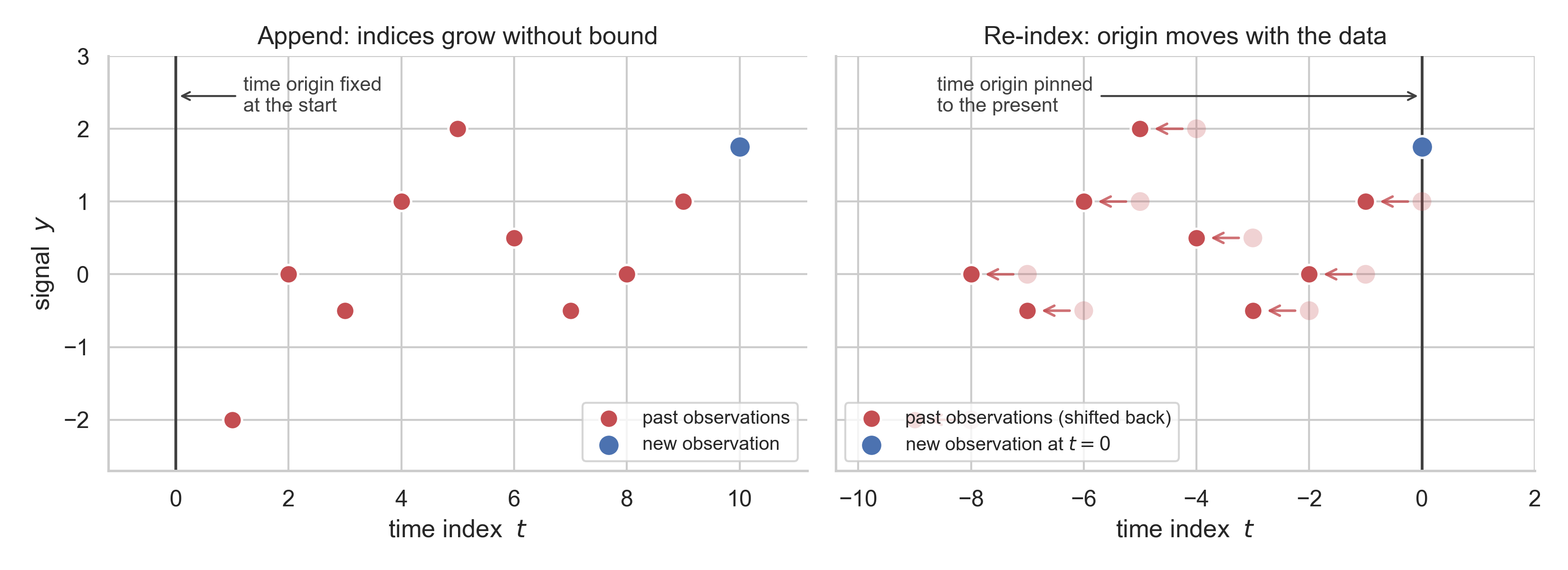
Intuitively, by both having longer-ago datapoints downweighted and keeping recent, high-weight datapoints close to \(t=0\), all the sums that make up the estimator saturate at certain values as \(t \to \infty\), rather than growing without limit. We work in this limiting case throughout: the steady state the estimator settles into once it has seen plenty of data. (This moving-origin construction is Brown’s “discounted least squares” — and the saturation is also exactly what you want if you ever have to run this estimator online, keeping a running estimate that you update as each observation comes in.)
With design vector \(f(j) = (1, -j)^\top\), the weighted normal equations are \(F\,(\hat \alpha, \hat\beta)^\top = g\) with
\[F = \sum_{j\ge 0} \lambda^j f(j) f(j)^\top, \qquad g = \sum_{j \ge 0} \lambda^j f(j)\, y_{t-j}.\]The estimator is linear in the data, \((\hat \alpha, \hat\beta)^\top = F^{-1} g\), so its covariance is \(\sigma^2\, F^{-1} K F^{-1}\) where \(K = \sum_j \lambda^{2j} f(j) f(j)^\top\) (the same matrix with \(\lambda \to \lambda^2\), because the weights get squared inside the variance). Everything is built from three geometric sums and their \(\lambda^2\) versions — these are the limiting values as \(t\to\infty\); at finite \(t\) each carries correction terms of order \(\lambda^t\), which die off quickly:
\[\sum_{j\ge0} \lambda^j = \frac{1}{1-\lambda}, \qquad \sum_{j\ge0} j\,\lambda^j = \frac{\lambda}{(1-\lambda)^2}, \qquad \sum_{j\ge0} j^2 \lambda^j = \frac{\lambda(1+\lambda)}{(1-\lambda)^3}.\]Reading off the elements of \(\sigma^2 F^{-1} K F^{-1}\) (a few lines of algebra, or one line of sympy) gives
\[\mathrm{Var}(\hat\beta_\lambda) = \frac{2(1-\lambda)^3}{(1+\lambda)^3}\,\sigma^2,\]and as a sanity check, the same machinery with the constant-only model \(f(j) = 1\) gives \(\mathrm{Var}(\bar y_\lambda) = \frac{1-\lambda}{1+\lambda}\,\sigma^2\), the level result from the main text. Both formulas match Monte Carlo simulation to within sampling error (the dots and dotted lines in the crossing figure above).
D. The level memory length without variances: average age
Brown’s original argument (1963, p. 107) doesn’t mention variance at all. The average age of the data in an exponentially weighted mean is
\[\bar j = \frac{\sum_j j\,\lambda^j}{\sum_j \lambda^j} = \frac{\lambda}{1-\lambda},\]while a sliding window of \(N\) points has ages \(0, 1, \ldots, N-1\), so average age \((N-1)/2\). Equating:
\[\frac{N-1}{2} = \frac{\lambda}{1-\lambda} \quad\Longrightarrow\quad N = \frac{1+\lambda}{1-\lambda}.\]Same answer as the variance match — for the level, the two notions of “equivalent window” coincide. (For the slope they would not, which is part of why the trend result is easy to miss.)
E. What if you don’t drop the \(-t_{\mathrm{mem}}\)?
The exact equivalent window solves the depressed cubic
\[N^3 - N = c, \qquad c = 6\left(\frac{1+\lambda}{1-\lambda}\right)^3,\]whose real root has a closed form, \(N = \tfrac{2}{\sqrt 3}\cosh\!\left(\tfrac13 \cosh^{-1}\!\big(\tfrac{3\sqrt3}{2}c\big)\right)\), though a perturbative correction to the cube root is helpful: writing \(N = c^{1/3}(1+\delta)\) and keeping first order gives
\[N \approx c^{1/3} + \frac{1}{3\,c^{1/3}}.\]Numbers:
| \(\lambda\) | \(t_{\mathrm{mem}}^{\mathrm{level}}\) | \(6^{1/3}(1+\lambda)/(1-\lambda)\) | exact root | error | with correction |
|---|---|---|---|---|---|
| 0.50 | 3.0 | 5.451 | 5.513 | −1.11% | 5.513 |
| 0.70 | 5.7 | 10.297 | 10.329 | −0.31% | 10.329 |
| 0.80 | 9.0 | 16.354 | 16.374 | −0.12% | 16.374 |
| 0.90 | 19.0 | 34.525 | 34.535 | −0.03% | 34.535 |
| 0.95 | 39.0 | 70.868 | 70.872 | −0.01% | 70.872 |
| 0.99 | 199.0 | 361.607 | 361.608 | −0.00% | 361.608 |
So the cube-root form is already within ~1% at \(\lambda = 0.5\) (a five-step memory!) and the one-term correction makes it exact for all practical purposes:
-
For example, financial time series are commonly modelled as stochastic processes, which are not differentiable: you cannot find a gradient as an infinitesimal rise-over-run calculation. ↩
-
A weighting that places all weight on a pair of datapoints will exactly obtain a rise-over-run estimate from doing weighted linear regression: with only two effectively-weighted points the fitted line passes through both of them (two free parameters, two points, zero residuals), so \(\beta\) is exactly the rise over the run — whatever the two weights are. ↩